Computing Periods
This chapter is about computing period maps associated to newforms. We assume you have read Chapters General Modular Symbols and Computing with Newforms and that you are familiar with abelian varieties at the level of [Ros86].
In Section The Period Map we introduce the period map and give some examples of situations in which computing it is relevant. Section Abelian Varieties Attached to Newforms is about how to use the period mapping to attach an abelian variety to any newform. In Section Extended Modular Symbols, we introduce extended modular symbols, which are the key computational tool for quickly computing periods of modular symbols. We turn to numerical computation of period integrals in Section Approximating Period Integrals, and in Section Speeding Convergence Using Atkin-Lehner we explain how to use Atkin-Lehner operators to speed convergence. In Section Computing the Period Mapping we explain how to compute the full period map with a minimum amount of work.
Section All Elliptic Curves of Given Conductor briefly sketches three approaches to computing all elliptic curves of a given conductor.
This chapter was inspired by [Cre97a], which contains
similar algorithms in the special case of a
newform  with
with  .
.
See also [Dok04] for algorithmic methods to compute
special values of very general  -functions, which can be used for
approximating
-functions, which can be used for
approximating  for arbitrary
  .
.
The Period Map
Let  be a subgroup of
  that contains
 for some
  , and
suppose
, and
suppose
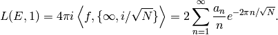
is a newform (see Definition Definition 9.9). In this chapter we describe how to approximately compute the complex period mapping
given by
as in Section Pairing Modular Symbols and Modular Forms. As an application, we can
approximate the special values  , for
, for  using
(?). We can also
compute the period lattice attached to a modular abelian variety,
which is an important step, e.g., in enumeration of
using
(?). We can also
compute the period lattice attached to a modular abelian variety,
which is an important step, e.g., in enumeration of
 -curves (see, e.g., [GLQ04]) or computation of
a curve whose Jacobian is a modular abelian variety
-curves (see, e.g., [GLQ04]) or computation of
a curve whose Jacobian is a modular abelian variety  (see, e.g., [Wan95]).
Abelian Varieties Attached to Newforms
Fix a newform  , where
  for some . Let
  be the
 -conjugates of
  , where acts via
its action on the Fourier coefficients, which are algebraic integers
(since they are the eigenvalues of matrices with integer entries).
Let
, where acts via
its action on the Fourier coefficients, which are algebraic integers
(since they are the eigenvalues of matrices with integer entries).
Let
(1)
be the subspace of cusp forms spanned by the
-conjugates of .
One can show using the results discussed in Section Atkin-Lehner-Li Theory
that the above sum is direct, i.e., that  has dimension
  .
.
The integration pairing induces a  -equivariant homomorphism

from modular symbols to the  -linear dual
  of .
Here acts on via
of .
Here acts on via  ,
and this homomorphism is -stable by Theorem 1.42.
The abelian variety attached to is the
quotient
,
and this homomorphism is -stable by Theorem 1.42.
The abelian variety attached to is the
quotient

Here  , and we include
the
, and we include
the  in the notation to emphasize that
these are integral modular symbols.
See [Shim59] for a proof that
in the notation to emphasize that
these are integral modular symbols.
See [Shim59] for a proof that  is an abelian variety (in particular,
 is a lattice, and
is equipped with a nondegenerate Riemann form).
is a lattice, and
is equipped with a nondegenerate Riemann form).
When  , we can also construct as a quotient
of the modular Jacobian
, we can also construct as a quotient
of the modular Jacobian  , so is an
abelian variety canonically defined over .
, so is an
abelian variety canonically defined over .
In general, we have an exact sequence

Remark 10.1
When , the abelian variety has a canonical structure of
abelian variety over . Moreover, there is a conjecture of Ribet
and Serre in [Rib92] that describes the simple abelian
varieties  over that should arise via this construction. In
particular, the conjecture is that is isogenous to some abelian
variety if and only if
over that should arise via this construction. In
particular, the conjecture is that is isogenous to some abelian
variety if and only if  is a number field
of degree
is a number field
of degree  . The abelian varieties have this property
since
. The abelian varieties have this property
since  embeds in
and the endomorphism ring over has degree at most
(see [Rib92] for details). Ribet proves that his
conjecture is a consequence of Serre’s conjecture
[Ser87] on modularity of mod
embeds in
and the endomorphism ring over has degree at most
(see [Rib92] for details). Ribet proves that his
conjecture is a consequence of Serre’s conjecture
[Ser87] on modularity of mod  odd irreducible
Galois representations (see Section Applications of Modular Forms). Much of Serre’s
conjecture has been proved by Khare and Wintenberger (not
published). In particular, it is a theorem that if is a simple
abelian variety over with a number field
of degree and if has good reduction at
odd irreducible
Galois representations (see Section Applications of Modular Forms). Much of Serre’s
conjecture has been proved by Khare and Wintenberger (not
published). In particular, it is a theorem that if is a simple
abelian variety over with a number field
of degree and if has good reduction at  , then is
isogenous to some abelian variety .
, then is
isogenous to some abelian variety .
Remark 10.2
When  , there is an object called a
Grothendieck motive that is attached to and has a canonical
“structure over “. See [Sch90].
, there is an object called a
Grothendieck motive that is attached to and has a canonical
“structure over “. See [Sch90].
Extended Modular Symbols
In this section, we extend the notion of modular
symbols to allows symbols of the form
 where
where  and
and  are
arbitrary elements of
are
arbitrary elements of  .
.
Definition 10.3
The abelian group sym{esM_k}
of extended modular symbols of weight  is the -span of symbols , with
  a homogeneous polynomial of degree
  with integer
coefficients, modulo the relations
with integer
coefficients, modulo the relations

and modulo any torsion.
Fix a finite index subgroup  .
Just as for usual modular symbols,
.
Just as for usual modular symbols,  is equipped with
an action of , and we
define the space of extended modular symbols of weight
for to be the quotient
is equipped with
an action of , and we
define the space of extended modular symbols of weight
for to be the quotient

The quotient  is torsion-free and fixed by .
The integration pairing extends naturally to a pairing
(2)
where we recall from (?) that  denotes
the space of antiholomorphic cusp forms.
Moreover, if
denotes
the space of antiholomorphic cusp forms.
Moreover, if
is the natural map, then  respects (2) in the sense that
for all
respects (2) in the sense that
for all  and
and  , we have
As we will see soon, it
is often useful to replace
 first by
  and then
by an equivalent sum
and then
by an equivalent sum  of symbols
 such that
 is easier to
compute numerically than
is easier to
compute numerically than  .
.
Let  be a Dirichlet character of modulus .
If
be a Dirichlet character of modulus .
If  , let
, let  .index{
 }
Let sym{esM_k(N,eps)} be the quotient of
}
Let sym{esM_k(N,eps)} be the quotient of
![\esM_k(N,\Z[\eps])](_images/math/0aaae27f21a39dae657b783b85f6bd036ec31e72.png) by the relations
by the relations  , for all
 ![x \in \sM_k(N,\Z[\eps])](_images/math/892898775d582cfee11afab4f1f4a74a423ecb5a.png) ,
,
 , and modulo any torsion.
Approximating Period Integrals
In this section we assume is a congruence subgroup
of that contains for some .
Suppose  , so
, so  and
and  is
an integer such that
is
an integer such that  ,
and consider the extended modular symbol
,
and consider the extended modular symbol
 .
Let
.
Let  denote
the integration pairing from Section Pairing Modular Symbols and Modular Forms.
Given an arbitrary cusp form
denote
the integration pairing from Section Pairing Modular Symbols and Modular Forms.
Given an arbitrary cusp form  ,
we have
,
we have
The reversal of summation and integration is justified because
the imaginary part of  is positive so that the sum
converges absolutely. The following
lemma is useful for computing the above infinite sum.
is positive so that the sum
converges absolutely. The following
lemma is useful for computing the above infinite sum.
Lemma 10.4
(3)
Proof
See Exercise 10.1
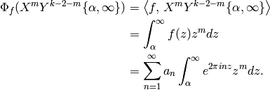
In practice we will usually be interested in computing the period map
 when
when  is a newform. Since is a
newform, there is a Dirichlet character such that
is a newform. Since is a
newform, there is a Dirichlet character such that  . The period map
 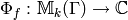 then
factors through the quotient
then
factors through the quotient  , so it suffices to
compute the period map on modular symbols in .
, so it suffices to
compute the period map on modular symbols in .
The following proposition is an analogue of [Cre97a, Prop. 2.1.1(5)].
Proposition 10.5
For any  ,
,  and
and  ,
we have the following relation in
,
we have the following relation in  :
:
Proof
By definition, if  is a modular symbol
and
is a modular symbol
and  , then
  .
Thus
.
Thus  , so
, so
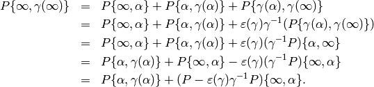
The second equality in the statement of the proposition now follows easily.
In the case of weight and trivial character,
the “error term”
(4)
vanishes since  is constant and
  . In general this term does
not vanish. However, we can suitably modify the formulas
found in [Cre97a, 2.10] and still obtain an algorithm
for computing period integrals.
. In general this term does
not vanish. However, we can suitably modify the formulas
found in [Cre97a, 2.10] and still obtain an algorithm
for computing period integrals.
Algorithm 10.6
Given , and
 presented as a
  -expansion to some precision,
this algorithm outputs an approximation to
the period integral
-expansion to some precision,
this algorithm outputs an approximation to
the period integral
 .
.
- Write
 , with
  ,
and set
,
and set  in Proposition Proposition 10.5.
 - Replacing
 by
by  if necessary,
we find that the imaginary parts of
if necessary,
we find that the imaginary parts of  and
and
 are both equal to the positive number
  .
. - Use (?) and Lemma 10.4 to compute the integrals that appear in Proposition Proposition 10.5.
It would be nice if the modular symbols
of the form  for and
were to generate a large subspace
of
for and
were to generate a large subspace
of  .
When and
.
When and  ,
Manin proved in [Man72]
that the map
,
Manin proved in [Man72]
that the map  sending to
  is a surjective
group homomorphism. When , the author
does not know a similar
group-theoretic statement. However, we have the following
theorem.
is a surjective
group homomorphism. When , the author
does not know a similar
group-theoretic statement. However, we have the following
theorem.
Theorem 10.7
Any element of  can be written in the form
for some  and
and  Moreover,
  and
and  can be chosen so that
 ,
so the error term (4) vanishes.
,
so the error term (4) vanishes.
Figure 10.1
“Transporting” a transportable modular symbol.
\begin{figure}
\begin{center}
\begin{picture}(230,150)(0,0)
\put(-10,10){\line(1,0){200}}
\put(10,10){\circle*{3}}
\put(10,0){`\infty`}
\qbezier(10,10)(50,40)(75,10)
\put(49,25){\vector(1,0){1}}
\put(45,28){`P`}
\put(75,10){\circle*{3}}
\put(75,0){`\gamma \infty`}
\qbezier(75,10)(130,50)(140,10)
\put(120,30){\vector(1,0){1}}
\put(115,34){`Q`}
\put(140,10){\circle*{3}}
\put(140,0){`\beta \infty`}
\put(20,90){\circle*{3}}
\put(17,96){`\alpha`}
\qbezier(20,90)(50,120)(55,60)
\put(40,100){\vector(1,0){1}}
\put(40,104){`P`}
\put(55,60){\circle*{3}}
\put(60,54){`\gamma \alpha`}
\qbezier(55,60)(70,180)(100,140)
\put(87,150){\vector(1,0){1}}
\put(85,154){`Q`}
\put(100,140){\circle*{3}}
\put(100,146){`\beta \alpha`}
\comment{
\qbezier(10,10)(-10,30)(10,50)
\qbezier(10,50)(40,70)(20,90)
\put(5,45){\vector(2,3){1}}
\qbezier(75,10)(90,30)(75,40)
\qbezier(75,40)(60,50)(55,60)
\put(69,45){\vector(1,-1){1}}
\put(80,35){\vector(-1,2){1}}
\qbezier(140,10)(160,30)(140,50)
\qbezier(140,50)(90,80)(110,90)
\qbezier(110,90)(130,100)(100,120)
\qbezier(100,120)(90,130)(100,140)
\put(110,90){\vector(-1,-1){1}}
}
\put(100,50){\vector(-1,4){10}}
\put(50,40){\vector(-1,4){10}}
\put(140,155){\parbox[t][4in][l]{2in}
{
The modular symbol


can be “transported” to
provided that

The author and Helena Verrill prove this theorem
in [SV01].
The condition
that the error term vanishes means that one can replace
 by any in the expression for the modular symbol
and obtain an equivalent modular symbol. For this reason,
we call such modular symbols transportable, as illustrated
in Figure 10.1.
by any in the expression for the modular symbol
and obtain an equivalent modular symbol. For this reason,
we call such modular symbols transportable, as illustrated
in Figure 10.1.
Note that in general not every element of the form
must lie in . However, if
 , then does lie in
. It would be interesting to know under what
circumstances is generated by symbols of the form
with . This sometimes fails for
odd; for example, when
, then does lie in
. It would be interesting to know under what
circumstances is generated by symbols of the form
with . This sometimes fails for
odd; for example, when  , the condition implies
that
, the condition implies
that  has an eigenvector with eigenvalue
  , and hence
is of finite order. When is even, the author can see no
obstruction to generating using such symbols.
, and hence
is of finite order. When is even, the author can see no
obstruction to generating using such symbols.
Speeding Convergence Using Atkin-Lehner
Let  .
Consider the Atkin-Lehner involution
.
Consider the Atkin-Lehner involution  on
on  ,
which is defined by
,
which is defined by
![W_N(f) &= N^{(2-k)/2} \cdot f|_{[w_N]_k}\\
&= N^{(2-k)/2} \cdot f\left(-\frac{1}{Nz}\right) \cdot N^{k-1} \cdot (Nz)^{-k}\\
&= N^{-k/2} \cdot z^{-k} \cdot f\left(-\frac{1}{Nz}\right).](_images/math/b255460f74e49812d36f14582958ab916207278b.png)
Here we take the positive square root if is odd.
Then  is an involution when is even.
There is an operator on modular symbols, which we also denote
, which is given by
and one has that if  and
and  , then

If is a Dirichlet character of modulus , then
the operator sends  to
to
 . Thus if
  ,
then preserves . In particular,
acts on
,
then preserves . In particular,
acts on  .
.
The next proposition shows how to compute the pairing
 under
certain restrictive assumptions.
It generalizes a result of [Cre97b] to
higher weight.
under
certain restrictive assumptions.
It generalizes a result of [Cre97b] to
higher weight.
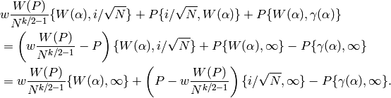
Proposition 10.8
Let  be a cusp form which is
an eigenform for the Atkin-Lehner operator
having eigenvalue
be a cusp form which is
an eigenform for the Atkin-Lehner operator
having eigenvalue  (thus and is even).
Then for any and any
, with the property that
(thus and is even).
Then for any and any
, with the property that  , we have
the following formula, valid for any
, we have
the following formula, valid for any  :
:
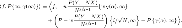
Here  .
.
Proof
By Proposition Proposition 10.5 our condition on
implies that  .
We describe the steps of the following computation below.
.
We describe the steps of the following computation below.
For the first equality, we break the path into three paths,
and in the second, we apply the  -involution to the first
term and use that the action of is compatible with
the pairing
-involution to the first
term and use that the action of is compatible with
the pairing  and that is an eigenvector
with eigenvalue .
In the following sequence of equalities we combine the first two terms
and break up the third; then we replace
and that is an eigenvector
with eigenvalue .
In the following sequence of equalities we combine the first two terms
and break up the third; then we replace  by
by
 and regroup:
A good choice for is
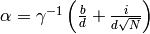 ,
so that
,
so that 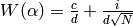 .
This maximizes the minimum of the imaginary parts
of and
.
This maximizes the minimum of the imaginary parts
of and  , which results in series that converge
more quickly.
, which results in series that converge
more quickly.
Let  .
The polynomial
.
The polynomial

satisfies  .
We obtained this formula by viewing
.
We obtained this formula by viewing  as
the
as
the  symmetric product of the -dimensional
space on which
symmetric product of the -dimensional
space on which  acts naturally. For example,
observe that since
acts naturally. For example,
observe that since  ,
the symmetric product of two eigenvectors for is an eigenvector
in
,
the symmetric product of two eigenvectors for is an eigenvector
in  having eigenvalue .
For the same reason, if
having eigenvalue .
For the same reason, if  , there need
not be a polynomial
, there need
not be a polynomial  such that
  .
One remedy is to choose another so that .
.
One remedy is to choose another so that .
Since the imaginary parts of the terms  , and
in the proposition are all relatively large, the sums
appearing at the beginning of Section Approximating Period Integrals converge
quickly if is small. It is important to
choose in Proposition Proposition 10.8 with small; otherwise
the series will converge very slowly.
, and
in the proposition are all relatively large, the sums
appearing at the beginning of Section Approximating Period Integrals converge
quickly if is small. It is important to
choose in Proposition Proposition 10.8 with small; otherwise
the series will converge very slowly.
Remark 10.9
Is there a generalization of Proposition Proposition 10.8
without the restrictions that and is even?
Another Atkin-Lehner Trick
Suppose  is an elliptic curve and let
  be the corresponding
-function. Let
be the corresponding
-function. Let  be the root number of , i.e.,
the sign of the functional equation for , so
be the root number of , i.e.,
the sign of the functional equation for , so
 , where
 .
Let
.
Let  be the modular form associated to
(which exists by [Wil95, BCDT01]).
If
be the modular form associated to
(which exists by [Wil95, BCDT01]).
If  , then
  (see Exercise 10.2). We have
If  , then
  . If
. If  , then
(5)
For more about computing with -functions of elliptic curves,
including a trick for computing quickly without directly
computing , see [Coh93, Section 7.5] and
[Cre97a, Section 2.11]. One can also find higher derivatives
 by a formula similar to (5) (see
[Cre97a, Section 2.13]). The methods in this chapter for
obtaining rapidly converging series are not just of computational
interest; see, e.g., [Gre83] for a nontrivial
theoretical application to the Birch and Swinnerton-Dyer conjecture.
by a formula similar to (5) (see
[Cre97a, Section 2.13]). The methods in this chapter for
obtaining rapidly converging series are not just of computational
interest; see, e.g., [Gre83] for a nontrivial
theoretical application to the Birch and Swinnerton-Dyer conjecture.
Computing the Period Mapping
Fix a newform  ,
where
for some .
Let be as in (1).
,
where
for some .
Let be as in (1).
Let  be any -linear map with the same kernel
as ; we call any such map a rational period mapping
associated to . Let be the period mapping associated
to the -conjugates of . We
have a commutative diagram
be any -linear map with the same kernel
as ; we call any such map a rational period mapping
associated to . Let be the period mapping associated
to the -conjugates of . We
have a commutative diagram
![\xymatrix{
{\sM_k(\Gamma;\Q)}\ar[dr]_{\Theta_f}\ar[rr]^{\Phi_f}
& & \Hom_\C(V_f,\C) \\
& V\ar@{^(->}[ur]^{i_f}
}](_images/math/7c49f38075eec0af4e770e6bd2f84eafa015ff03.png)
Recall from Section Abelian Varieties Attached to Newforms that the cokernel of
is the abelian variety .
The Hecke algebra acts on the linear dual

by  .
Let
.
Let  be the kernel of the
ring homomorphism
be the kernel of the
ring homomorphism ![\T\ra \Z[a_2, a_3, \ldots]](_images/math/1ccb1927f1cb8be143710be54e9978518f4c19ba.png) that sends
that sends  to
to  .
Let
.
Let
![\sM_k(\Gamma;\Q)^*[I] = \{\vphi \in \sM_k(\Gamma;\Q)^* : t \vphi =
0 \text{ all }t \in I\}.](_images/math/b54462247e606e9e2a16edc558aaa8e729835da4.png)
Since is a newform, one can show that
![\sM_k(\Gamma;\Q)^*[I]](_images/math/f6079cc6c9d622784f6e07d328d6f7f54c80e09d.png) has dimension .
Let
has dimension .
Let  be a basis
for , so
be a basis
for , so

We can thus compute  , hence a choice of
  .
To compute , it remains to compute
.
To compute , it remains to compute  .
.
Let  denote the space of cusp forms with
-expansion in
denote the space of cusp forms with
-expansion in ![\Q[[q]]](_images/math/59f0eca8d1174db9767b50a081db45c7b035541a.png) .
By Exercise 10.3
.
By Exercise 10.3
![S_k(\Gamma; \Q)[I] = S_k(\Gamma)[I] \cap \Q[[q]]](_images/math/73a84e91f848138fd9a6499c645b6f69bf407d2b.png)
is a -vector space of dimension .
Let  be a basis for this -vector space.
We will compute with respect to the basis of
be a basis for this -vector space.
We will compute with respect to the basis of
![\Hom_\Q(S_k(\Gamma;\Q)[I];\C)](_images/math/6dc90eb687d76e37c313a1cc20cea43674570d5e.png) dual to this basis.
Choose elements
dual to this basis.
Choose elements  with the following properties:
- Using Proposition Proposition 10.5 or Proposition Proposition 10.8,
it is possible to compute the period integrals
 ,
,  ,
efficiently.
,
efficiently. - The
 elements
  and
and  for
for  span a space of dimension (i.e., they span
  ).
).
Given this data, we can compute

and

We break the integrals into real and imaginary parts because this
increases the precision of our answers.
Since the vectors  and
and  ,
,  , span
 , we have computed .
Remark 10.10
We want to find symbols  satisfying the
conditions of Proposition Proposition 10.8. This is usually possible
when is very small, but in practice it is difficult when is large.
satisfying the
conditions of Proposition Proposition 10.8. This is usually possible
when is very small, but in practice it is difficult when is large.
Remark 10.11
The above strategy was motivated by [Cre97a, Section 2.10].
All Elliptic Curves of Given Conductor
Using modular symbols and the period map, we can compute all elliptic
curves over of conductor , up to isogeny. The algorithm in
this section gives all modular elliptic curves (up to isogeny),
i.e., elliptic curves attached to modular forms, of conductor .
Fortunately, it is now known by
[Wil95, BCDT01, TW95]
that every
elliptic curve over is modular, so the procedure of this section
gives all elliptic curves (up to isogeny) of given conductor. See
[Cre06] for a nice historical discussion of this
problem.
Algorithm 10.12
Given  , this
algorithm outputs equations for all
elliptic curves of conductor , up to isogeny.
, this
algorithm outputs equations for all
elliptic curves of conductor , up to isogeny.
[Modular Symbols] Compute
 using Section Explicitly Computing .
[Find Rational Eigenspaces] Find the
-dimensional eigenspaces  in
in
 that correspond to elliptic curves.
Do not use the algorithm for decomposition from
Section Decomposing Spaces under the Action of Matrix, which is too complicated
and gives more information than we need. Instead, for the first
few primes
that correspond to elliptic curves.
Do not use the algorithm for decomposition from
Section Decomposing Spaces under the Action of Matrix, which is too complicated
and gives more information than we need. Instead, for the first
few primes  , compute all eigenspaces
  , where
 runs through integers with
  .
Intersect these eigenspaces to find the eigenspaces that
correspond to elliptic curves. To find just the new ones,
either compute the degeneracy maps to lower level or find
all the rational eigenspaces of all levels that strictly
divide and exclude them.
.
Intersect these eigenspaces to find the eigenspaces that
correspond to elliptic curves. To find just the new ones,
either compute the degeneracy maps to lower level or find
all the rational eigenspaces of all levels that strictly
divide and exclude them.[Find Newforms] Use Algorithm 9.14 to compute to some precision each newform
![f=\sum_{n=1}^{\infty} a_n q^n \in \Z[[q]]](_images/math/e47ac17aa654a62780a66740ace793fdf4389e20.png) associated
to each eigenspace found in step (2).
associated
to each eigenspace found in step (2).[Find Each Curve] For each newform
found in step (3), do the following:[Period Lattice] Compute the corresponding period lattice
 by computing the image of ,
as described in Section Computing the Period Mapping.
by computing the image of ,
as described in Section Computing the Period Mapping.[Compute
 ]
Let
]
Let  . If
. If  , swap
 and
and  , so
, so  .
By successively applying generators of ,
we find an equivalent element
.
By successively applying generators of ,
we find an equivalent element  in
in  , i.e.,
 and
and  .
.[
 -invariants] Compute the invariants
  and
and  of the lattice
  using the following
rapidly convergent series:
using the following
rapidly convergent series: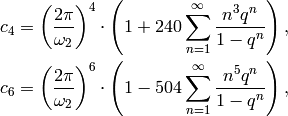
where
 , where is as in step
(b).
A theorem of Edixhoven
(that the Manin constant is an integer) implies that
the invariants and of are integers,
so it is only necessary to compute to large
precision to completely determine them.
, where is as in step
(b).
A theorem of Edixhoven
(that the Manin constant is an integer) implies that
the invariants and of are integers,
so it is only necessary to compute to large
precision to completely determine them.[Elliptic Curve] An elliptic curve with invariants
and is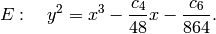
[Prove Correctness] Using Tate’s algorithm, find the conductor of
. If the conductor is not , then recompute and
using more terms of and real numbers
to larger precision, etc. If the conductor is ,
compute the coefficients  of the modular form
  attached to the elliptic curve , for
  .
Verify that
.
Verify that  , where
  are the coefficients
of . If this equality holds, then must be isogenous
to the elliptic curve attached to , by the Sturm
bound (Theorem 9.18) and Faltings’s isogeny theorem.
If the equality fails for some , recompute and
to larger precision.
are the coefficients
of . If this equality holds, then must be isogenous
to the elliptic curve attached to , by the Sturm
bound (Theorem 9.18) and Faltings’s isogeny theorem.
If the equality fails for some , recompute and
to larger precision.
There are numerous tricks to optimize the above algorithm.
For example, often one can work separately with
 and
and
 and
get enough information to find , up to isogeny
(see [Cre97b]).
and
get enough information to find , up to isogeny
(see [Cre97b]).
Once we have one curve from each isogeny class of curves of
conductor , we find each curve in each isogeny class (which is
another interesting problem discussed in [Cre97a]), hence
all curves of conductor . If  is an elliptic curve, then any
curve isogenous to is isogenous via a chain of isogenies of prime
degree. There is an a priori bound on the degrees of these
isogenies due to Mazur. Also, there are various methods for finding
all isogenies of a given degree with domain . See
[Cre97a, Section 3.8] for more details.
is an elliptic curve, then any
curve isogenous to is isogenous via a chain of isogenies of prime
degree. There is an a priori bound on the degrees of these
isogenies due to Mazur. Also, there are various methods for finding
all isogenies of a given degree with domain . See
[Cre97a, Section 3.8] for more details.
Finding Curves:  -Integral Points
In this section we briefly survey an alternative approach to finding curves of a given conductor by finding integral points on other elliptic curves.
Cremona and others have developed a complementary
approach to the problem of computing all elliptic curves of given
conductor (see [CL04]). Instead of computing all
curves of given conductor, we instead consider the seemingly more
difficult problem of finding all curves with good reduction outside a
finite set of primes. Since one can compute the conductor of a
curve using Tate’s algorithm
[Tat75, Cre97a, Section 3.2],
if we know all curves with good reduction
outside , we can find all curves of conductor by letting be
the set of prime divisors of .
There is a strategy for finding all curves with good reduction
outside . It is not an algorithm, in the sense
that it is always guaranteed to terminate (the modular symbols method
above is an algorithm), but in practice it often works. Also,
this strategy makes sense over any number field, whereas the modular
symbols method does not (there are generalizations of modular
symbols to other number fields).
Fix a finite set of primes of a number field  . It is a theorem
of Shafarevich that there are only finitely many elliptic curves with
good reduction outside (see [Sil82, Section IX.6]). His
proof uses that the group of -units in is finite and Siegel’s
theorem that there are only finitely many -integral points on an
elliptic curve. One can make all this explicit, and sometimes in
practice one can compute all these -integral points.
. It is a theorem
of Shafarevich that there are only finitely many elliptic curves with
good reduction outside (see [Sil82, Section IX.6]). His
proof uses that the group of -units in is finite and Siegel’s
theorem that there are only finitely many -integral points on an
elliptic curve. One can make all this explicit, and sometimes in
practice one can compute all these -integral points.
The problem of finding all elliptic curves with good reduction outside
of can be broken into several subproblems, the main ones being
determine the following finite subgroup of
 :
:
find all
-integral points on certain elliptic curves
 .
.
In [CL04], there is one example, where they find all
curves of conductor  by finding all curves
with good reduction outside
by finding all curves
with good reduction outside  . They finds
  curves of
conductor
curves of
conductor  that divide into
  isogeny classes.
(Note that
isogeny classes.
(Note that  .)
.)
Finding Curves: Enumeration
One can also find curves by simply enumerating Weierstrass equations.
For example, the paper [SW02] discusses a database
that the author and Watkins created that contains hundreds of millions
of elliptic curves. It was constructed by enumerating Weierstrass
equations of a certain form. This database does not contain
every curve of each conductor included in the database. It is,
however, fairly complete in some cases. For example, using the Mestre
method of graphs [Mes86], we verified in [JBS03] that
the database contains all elliptic curve of prime conductor  , which implies that the smallest conductor
rank
, which implies that the smallest conductor
rank  curve is composite.
Exercises
Exercise 10.1
Prove Lemma 10.4.
Exercise 10.2
Suppose  is a newform
and that . Let
is a newform
and that . Let  .
Prove that
.
Prove that

[Hint: Show that  .
Then substitute
.
Then substitute  for
for  .]
.]
Exercise 10.3
Let ![f=\sum a_n q^n \in \C[[q]]](_images/math/fa1649af4150949bd79efb718570d0a9c26b7045.png) be a power
series whose coefficients together generate a number field of
degree over . Let be the complex vector space spanned
by the -conjugates of .
be a power
series whose coefficients together generate a number field of
degree over . Let be the complex vector space spanned
by the -conjugates of .
- Give an example to show that need not have dimension .
- Suppose has dimension . Prove that
![V_f \cap
\Q[[q]]](_images/math/b67bd75f7079035a09a8e8f97b683787f619bc1c.png) is a -vector space of dimension .
is a -vector space of dimension .
Exercise 10.4
Find an elliptic curve of conductor  using Section
All Elliptic Curves of Given Conductor.
using Section
All Elliptic Curves of Given Conductor.
Table Of Contents
- Computing Periods
Previous topic
Next topic
Solutions to Selected Exercises