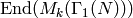
Eisenstein Series and Bernoulli Numbers
We introduce generalized Bernoulli numbers attached to Dirichlet
characters and give an algorithm to enumerate the Eisenstein series
in  .
.
The Eisenstein Subspace
Let  be the space of modular forms of weight
 for
for  , and let
  be the Hecke algebra
acting on , which is the subring of
be the Hecke algebra
acting on , which is the subring of
 generated by all Hecke operators.
Then there is a -module decomposition
generated by all Hecke operators.
Then there is a -module decomposition

where  is the subspace of modular forms that vanish
at all cusps and
is the subspace of modular forms that vanish
at all cusps and  is the
Eisenstein subspace, which
is uniquely determined by this decomposition.
The above decomposition
induces a decomposition of
is the
Eisenstein subspace, which
is uniquely determined by this decomposition.
The above decomposition
induces a decomposition of  and of
, for any Dirichlet character
and of
, for any Dirichlet character  of modulus
  .
.
Generalized Bernoulli Numbers
Suppose is a Dirichlet character of modulus over  .
Leopoldt [Leo58] defined generalized Bernoulli
numbers attached to .
.
Leopoldt [Leo58] defined generalized Bernoulli
numbers attached to .
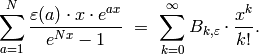
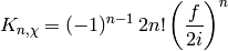
Definition 5.1
We define the generalized Bernoulli numbers  attached to by the following
identity of infinite series:
attached to by the following
identity of infinite series:
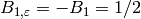
If is the trivial character of modulus  and
and  are as in Section Examples of Modular Forms of Level 1, then
 , except when
  , in which case
 (see Exercise 5.2).
Algebraically Computing Generalized Bernoulli Numbers
Let  denote the field generated by the image
of the character ; thus is the cyclotomic
extension
denote the field generated by the image
of the character ; thus is the cyclotomic
extension  , where
  is the order of .
Algorithm 5.2
Given an integer  and any
Dirichlet character with modulus , this algorithm computes
the generalized Bernoulli numbers
and any
Dirichlet character with modulus , this algorithm computes
the generalized Bernoulli numbers  , for
, for  .
.
Compute
![g \set x/(e^{Nx}-1) \in \Q[[x]]](_images/math/e3ccc02e86e79f0780606f32c3509996e9dc4686.png) to precision
to precision
 by computing
 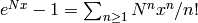 to precision
  and computing the inverse
 , then multiplying by
  .
.For each
 , compute
![f_a \set g \cdot e^{ax}\in\Q[[x]]](_images/math/742c91cb0d08254714f2d9d9b21cb609fd7718b1.png) , to precision .
This requires computing
, to precision .
This requires computing 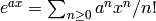 to
precision . (Omit computation of
to
precision . (Omit computation of  if
if  since then
  .)
.)Then for
, we have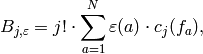
where
 is the coefficient of
  in
in  .
.
Note that in steps (1) and (2) we compute the
power series doing arithmetic only in ![\Q[[x]]](_images/math/562f19fccc5907ba1d5ca3413336c3eb4c8028d5.png) , not in
, not in
![\Q(\eps)[[x]]](_images/math/e65d36d686f8eb0476968bc1d6dde7b264effd93.png) , which could be much less efficient if has
large order. In step (1) if is huge,
we could compute the inverse using
asymptotically fast arithmetic and
Newton iteration.
, which could be much less efficient if has
large order. In step (1) if is huge,
we could compute the inverse using
asymptotically fast arithmetic and
Newton iteration.
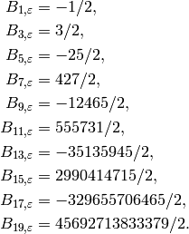
Example 5.3
The nontrivial character with modulus  has order
  and takes values in
  . The Bernoulli
numbers for even are all
. The Bernoulli
numbers for even are all  and for odd
they are
and for odd
they are
Example 5.4
The generalized Bernoulli numbers
need not be in . Suppose is the mod  character
such that
character
such that 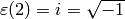 . Then
  for even
and
for even
and
Example 5.5
We use Sage to compute some of the above generalized Bernoulli numbers.
First we define the character and verify that  (note that
in Sage zeta4 is
(note that
in Sage zeta4 is  ).
).
sage: G = DirichletGroup(5)
sage: e = G.0
sage: e(2)
zeta4
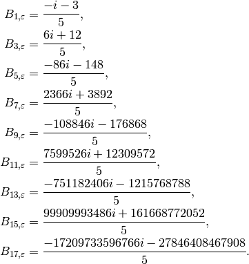
We compute the Bernoulli number  .
.
sage: e.bernoulli(1)
-1/5*zeta4 - 3/5
We compute  .
.
sage: e.bernoulli(9)
-108846/5*zeta4 - 176868/5
Proposition 5.6
If  and
and  , then .
Proof
See Exercise 5.3.
Computing Generalized Bernoulli Numbers Analytically
This section, which was written jointly with Kevin McGown, is about a way to compute generalized Bernoulli numbers, which is similar to the algorithm in Section Fast Computation of Bernoulli Numbers.
Let  be a primitive Dirichlet character
modulo its conductor
be a primitive Dirichlet character
modulo its conductor  .
Note from the definition of Bernoulli numbers that
if
.
Note from the definition of Bernoulli numbers that
if  , then
(1)
For any character , we define the Gauss sum  as
as
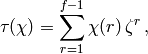
where 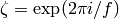 is the principal
  root of unity.
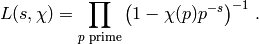
The Dirichlet
root of unity.
The Dirichlet  -function for for
  is
is
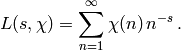
In the right half plane 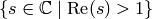 this function is analytic, and because is
multiplicative, we have the Euler product representation
this function is analytic, and because is
multiplicative, we have the Euler product representation
(2)
We note (but will not use) that through analytic continuation  can be extended to a meromorphic function on the entire complex plane.
If is a nonprincipal primitive Dirichlet character of
conductor such that 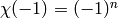 , then (see, e.g.,
[Wan82])
, then (see, e.g.,
[Wan82])
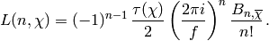
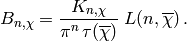
Solving for the Bernoulli number yields
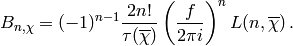
This allows us to give decimal approximations for  .
It remains to compute exactly (i.e., as an algebraic integer).
To simplify the above expression, we define
.
It remains to compute exactly (i.e., as an algebraic integer).
To simplify the above expression, we define
and write
(3)
Note that we can compute  exactly in the field
 .
.
The following result
identifies the denominator of .
Theorem 5.7
Let and be as above, and
define an integer  as follows:
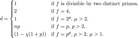
Then  is integral.
To compute the algebraic integer  , and we compute
 to very high precision using the Euler product
(2) and the formula (3). We carry out the
same computation for each of the
to very high precision using the Euler product
(2) and the formula (3). We carry out the
same computation for each of the  conjugates of
, which by (1) yields the conjugates of
. We can then write down the characteristic
polynomial of to very high precision and
recognize the coefficients as rational integers. Finally, we determine
which of the roots of the characteristic polynomial is
conjugates of
, which by (1) yields the conjugates of
. We can then write down the characteristic
polynomial of to very high precision and
recognize the coefficients as rational integers. Finally, we determine
which of the roots of the characteristic polynomial is  by approximating them all numerically to high precision
and seeing which is closest to our numerical approximation to
. The details are similar
to what is explained in Section Fast Computation of Bernoulli Numbers.
by approximating them all numerically to high precision
and seeing which is closest to our numerical approximation to
. The details are similar
to what is explained in Section Fast Computation of Bernoulli Numbers.
Explicit Basis for the Eisenstein Subspace
Suppose and  are primitive Dirichlet characters with
conductors and
are primitive Dirichlet characters with
conductors and  , respectively.
Let
, respectively.
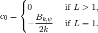
Let
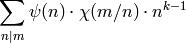
(4)![E_{k,\chi,\psi}(q) = c_0 + \sum_{m \geq 1} \left(
\sum_{n|m} \psi(n) \cdot \chi(m/n) \cdot n^{k-1}\right) q^{m}
\in \Q(\chi, \psi)[[q]],](_images/math/1a68b633092788869bfb04f62800fc4f2b2071f8.png)
where
Note that when  and
and  , then
  ,
where
,
where  is from Chapter Modular Forms.
Miyake proves statements that imply the following in [Miy89, Ch. 7].
Theorem 5.8
Suppose  is a positive integer and , are as above
and that is a positive integer such that
is a positive integer and , are as above
and that is a positive integer such that  .
Except when
.
Except when  and , the power series
 defines an element of
 .
If , ,
.
If , ,  , and
, and  , then
 is a modular form in
  .
.
Theorem 5.9
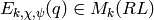
The Eisenstein series in  coming from
Theorem 5.8 with
coming from
Theorem 5.8 with  and
and  form a basis for the
Eisenstein subspace
form a basis for the
Eisenstein subspace  .
.
Theorem 5.10
The Eisenstein series
 defined above
are eigenforms (i.e., eigenvectors for all Hecke operators
defined above
are eigenforms (i.e., eigenvectors for all Hecke operators  ).
Also , for , is an eigenform.
).
Also , for , is an eigenform.
Since  is normalized so the coefficient
of
is normalized so the coefficient
of  is , the eigenvalue of
  is the coefficient
of  (see Proposition 9.10).
Also for
(see Proposition 9.10).
Also for  with prime, the coefficient of
is ,
with prime, the coefficient of
is ,  for
for  , and
, and  .
.
Algorithm 5.11
Given a weight and a Dirichlet character of modulus ,
this algorithm computes a basis for the Eisenstein
subspace of to precision  .
.
1. [Weight Trivial Character?] If and  , output the
Eisenstein series
, output the
Eisenstein series  , for each divisor
  with
with  , and then terminate.
- [Empty Space?] If
 , output the empty list.
 - [Compute Dirichlet Group] Let
 be the
group of Dirichlet characters with values in ,
where is the exponent of
be the
group of Dirichlet characters with values in ,
where is the exponent of  .
. - [Compute Conductors] Compute the
conductor of every element of
 using
Algorithm 4.19.
using
Algorithm 4.19. - [List Characters ] Form a list
 of all Dirichlet characters
  such that
 divides .
 - [Compute Eisenstein Series] For each character in ,
let
 and compute
 for each divisor of
 . Here we compute
 using (4) and
Algorithm 5.2.
using (4) and
Algorithm 5.2.
Remark 5.12
Algorithm 5.11 is what is currently used in Sage. It might be better to first reduce to the prime power case by writing all characters as a product of local characters and combine steps (4) and (5) into a single step that involves orders. However, this might make things more obscure.
Example 5.13
The following is a basis of Eisenstein series
for  .
.
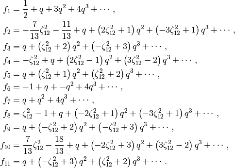
We computed it as follows:
sage: E = EisensteinForms(Gamma1(13),2)
sage: E.eisenstein_series()
We can also compute the parameters  that
define each series:
that
define each series:
sage: e = E.eisenstein_series()
sage: for e in E.eisenstein_series():
...       print e.parameters()
...
([1], [1], 13)
([1], [zeta6], 1)
([zeta6], [1], 1)
([1], [zeta6 - 1], 1)
([zeta6 - 1], [1], 1)
([1], [-1], 1)
([-1], [1], 1)
([1], [-zeta6], 1)
([-zeta6], [1], 1)
([1], [-zeta6 + 1], 1)
([-zeta6 + 1], [1], 1)
Exercises
Exercise 5.1
Suppose  and
and  are diagonalizable linear transformations of a
finite-dimensional vector space over an algebraically closed
field
are diagonalizable linear transformations of a
finite-dimensional vector space over an algebraically closed
field  and that
  . Prove there is a basis for so that
the matrices of and with respect to that basis are both
simultaneously diagonal.
. Prove there is a basis for so that
the matrices of and with respect to that basis are both
simultaneously diagonal.
Exercise 5.2
If is the trivial character of modulus and are as
in Section Examples of Modular Forms of Level 1, then ,
except when , in which case .
Exercise 5.3
Prove that for if , then
 .
.
Exercise 5.4
Show that the dimension of the Eisenstein subspace
 is
is  by finding a basis of series
 . You do not have to write down the
-expansions of the series, but you do have to figure out which
. You do not have to write down the
-expansions of the series, but you do have to figure out which
 to use.