Finding Square Roots
We return in this section to the question of computing square roots.
If  is a field in which
  , and
, and
 , with
  ,
then
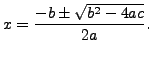
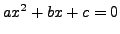
the solutions to the quadratic equation
,
then
the solutions to the quadratic equation
 are
are
Now assume
 , with
  an odd prime. Using
Theorem 4.1.7, we can decide whether or not
an odd prime. Using
Theorem 4.1.7, we can decide whether or not  is a
perfect square in
is a
perfect square in
 , and hence whether or not
has a solution in
. However
Theorem 4.1.7 says nothing about how to actually find
a solution when there is one.
Also, note that for this problem we do not need the
full quadratic reciprocity law; in practice to
decide whether an element of
is
a perfect square Proposition 4.2.1 is quite fast,
in view of Section 2.3.
, and hence whether or not
has a solution in
. However
Theorem 4.1.7 says nothing about how to actually find
a solution when there is one.
Also, note that for this problem we do not need the
full quadratic reciprocity law; in practice to
decide whether an element of
is
a perfect square Proposition 4.2.1 is quite fast,
in view of Section 2.3.
Suppose
 is a nonzero quadratic residue.
If
is a nonzero quadratic residue.
If
 then
then
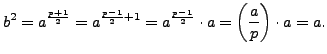
 is a square root of
  because
We can compute  in time polynomial in the number of digits of
using the powering algorithm of Section 2.3.
in time polynomial in the number of digits of
using the powering algorithm of Section 2.3.
Suppose next that
 .
Unfortunately, we do not know a deterministic algorithm
that takes as input
and
, outputs
a square root of
modulo
when one exists,
and is polynomial-time in
.
Unfortunately, we do not know a deterministic algorithm
that takes as input
and
, outputs
a square root of
modulo
when one exists,
and is polynomial-time in  .
.
Remark 4.5
There is an algorithm due to Schoof [#!schoof:sqrt!#] that computes
the square root of
in time
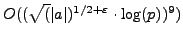
. This beautiful algorithm (which makes use of elliptic
curves) is not polynomial time in the sense described above since
for large
it takes exponentially longer than for small
.
We next describe a probabilistic algorithm to
compute a square root of
modulo
, which is very quick
in practice.
Recall the definition of ring from Definition 2.1.3.
We will also need the notion of ring homomorphism and isomorphism.
Definition 4.5 (Homomorphism of Rings)
Let

and

be rings.
A
homomorphism of rings

is a map such that for all

we have
An
isomorphism
of rings is a
ring homomorphism that is bijective.
Consider the (quotient) ring
defined as follows.
We have
with multiplication defined by
Here  corresponds to the class of
  in the quotient ring.
SAGE Example 4.5
We define and work with the quotient ring
above
in SAGE as follows (for

):
sage: S.<x> = PolynomialRing(GF(13))
sage: R.<alpha> = S.quotient(x^2 - 3)
sage: (2+3*alpha)*(1+2*alpha)
7*alpha + 7
Let
and  be the square roots of
in
(though we cannot easily
compute
and
yet, we can consider them in order
to deduce an algorithm to find them).
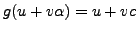
We have ring homomorphisms
be the square roots of
in
(though we cannot easily
compute
and
yet, we can consider them in order
to deduce an algorithm to find them).
We have ring homomorphisms
 and
and
 given by
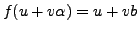 and
and
 .
Together these define a ring isomorphism
.
Together these define a ring isomorphism
given by
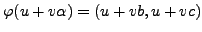 .
Choose in some way a random element
.
Choose in some way a random element  of
of
 , and
define
, and
define
 by
by
where we compute
 quickly
using an analogue of the
binary powering algorithm of Section 2.3.2.
If
quickly
using an analogue of the
binary powering algorithm of Section 2.3.2.
If  we try again with another random
. If
we try again with another random
. If  we can
quickly find the desired square roots
and
as follows. The
quantity
we can
quickly find the desired square roots
and
as follows. The
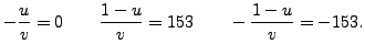
quantity  is a
is a  power in
, so it equals
either 0
,
power in
, so it equals
either 0
,  , or
, or  , so
, so  ,
,  , or
, or  ,
respectively. Since we know
,
respectively. Since we know  and
and  we can try each of
  ,
, and
and see which is a square root of
.
,
, and
and see which is a square root of
.
Example 4.5
Continuing Example
4.1.8,
we find a square root of

modulo

.
We apply the algorithm described above in the case
.
We first choose the random

and find that
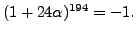
The coefficient of
in the power is
0
, and we try again with

.
This time we have
.
The inverse of

in

is

, so we consider the
following three possibilities for a square root of
:
Thus
and

are the square roots of
in
.
SAGE Example 4.5
We implement the above algorithm in SAGE and illustrate it
with some examples.
sage: def find_sqrt(a, p):
...    assert (p-1)%4 == 0
...    assert legendre_symbol(a,p) == 1
...    S.<x> = PolynomialRing(GF(p))
...    R.<alpha> = S.quotient(x^2 - a)
...    while True:
...        z = GF(p).random_element()
...        w = (1 + z*alpha)^((p-1)//2)
...        (u, v) = (w[0], w[1])
...        if v != 0: break
...    if (-u/v)^2 == a: return -u/v
...    if ((1-u)/v)^2 == a: return (1-u)/v
...    if ((-1-u)/v)^2 == a: return (-1-u)/v
...
sage: b = find_sqrt(3,13)
sage: b                        # random: either 9 or 3
9
sage: b^2
3
sage: b = find_sqrt(3,13)
sage: b                        # see, it's random
4
sage: find_sqrt(5,389)         # random: either 303 or 86
303
sage: find_sqrt(5,389)         # see, it's random
86
William
2007-06-01